Visualizing CoNLL NER Embeddings

I was thinking about NER tagsets recently – which tags should be included, what distinctions matter, where there is overlap – and it occurred to me that a visualization of the embeddings of each entity phrase could help shed some light.

You can click on each image for an ✨ interactive visualization ✨, or read farther for details and observations.

Embedding Entities

As with every other researcher for the past 19 years, the term “NER” makes me reflexively reach for CoNLL-2003 English dataset, with tagset: Person, Organization, Location, and Miscellaneous. Using the training set, I got the BERT embeddings (specifically distilroberta-base) for each labeled span (summing constituent subwords), and reduced to 2 dimensions with T-SNE. I repeated this process 6 times: one for each of the 4 labels, then 2 different plots with all labels but distinct coloring.

In one of the ALL plots, I colored according to label. In all others, I categorized using properties of each entity, assigning the first applicable category in this order: if it was preceded by a left parenthesis (paren), if it consisted of all capitals (all_caps), if it was the first token in a sentence (initial), and a catch-all category (plain). For the Location plot, I subdivided plain into LOC (if it was preceded by a preposition like “in” or “near”) and GPE (all others).

Observations

There are lots of interesting things to notice, I’ve written down a few below.

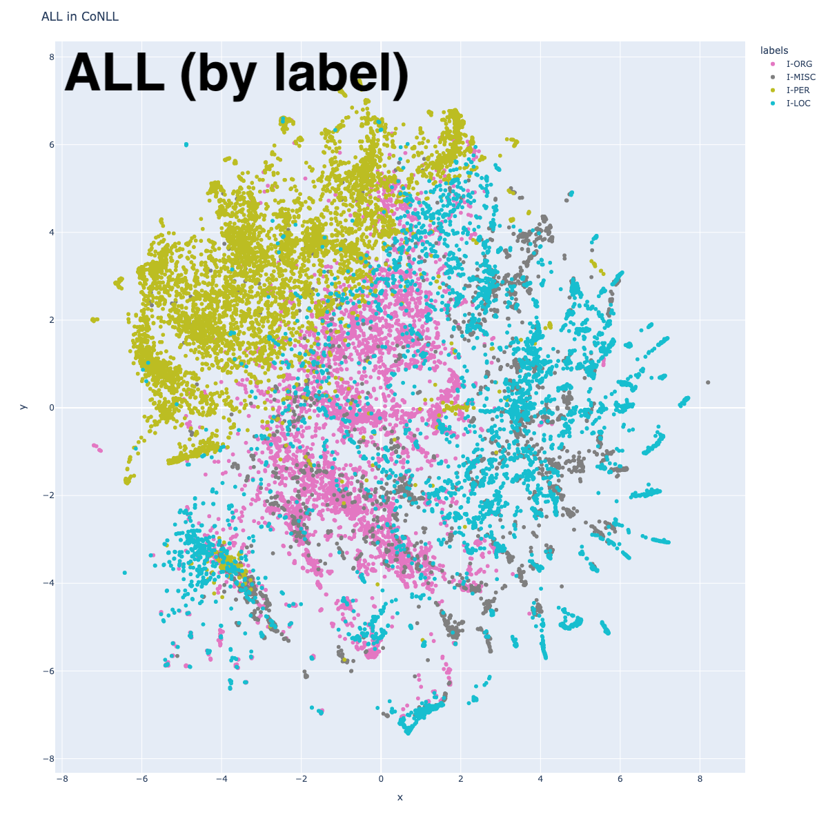
In the ALL-by-label plot, different areas for each label are apparent. Interestingly, Person is the most distinct, and while Organization and Location have central areas of density, the boundaries are less clear. Miscellaneous, on the other hand, seems to exist in the same spaces as Organization and Location. This will be explored more in a later section.

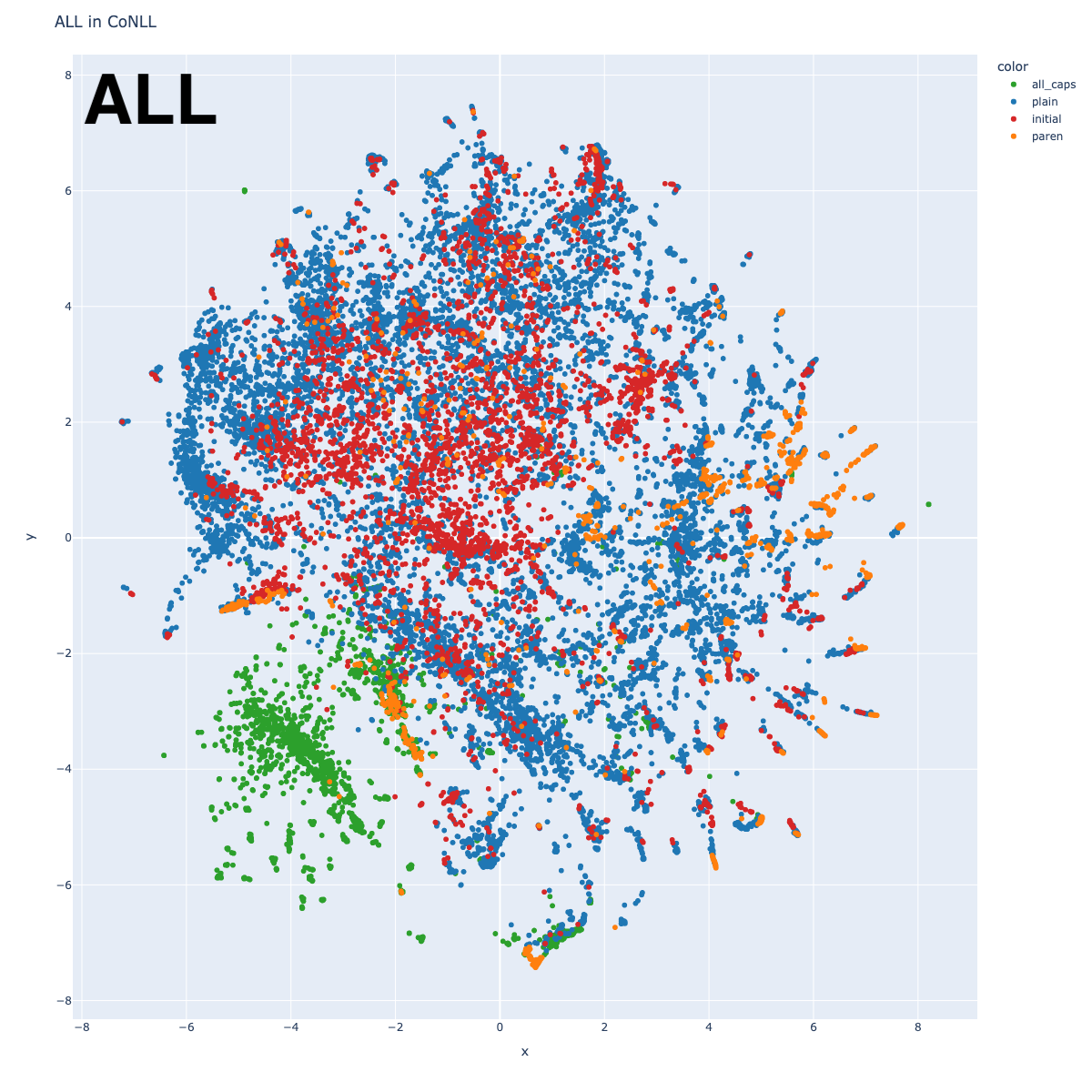
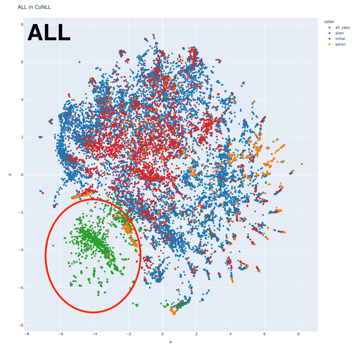There’s an odd island with center around (-4, -4). This becomes clearer when we look at the plot with the alternate coloring: that entire island is green, indicating that those entities are all capitalized. Unsurprisingly, each individual label plot shows a similar pattern.

Why are these all grouped together? It could be that BERT relies heavily on orthography, but it could also be an anomaly of the dataset, in which certain types of sentences are capitalized. Most points in this cluster represent document metadata strings, identifying location and date (“CALGARY 1996-08-23”, “BOMBAY 1996-08-22”) and some are document titles (“LOMBARDI WINS THIRD STAGE…”).

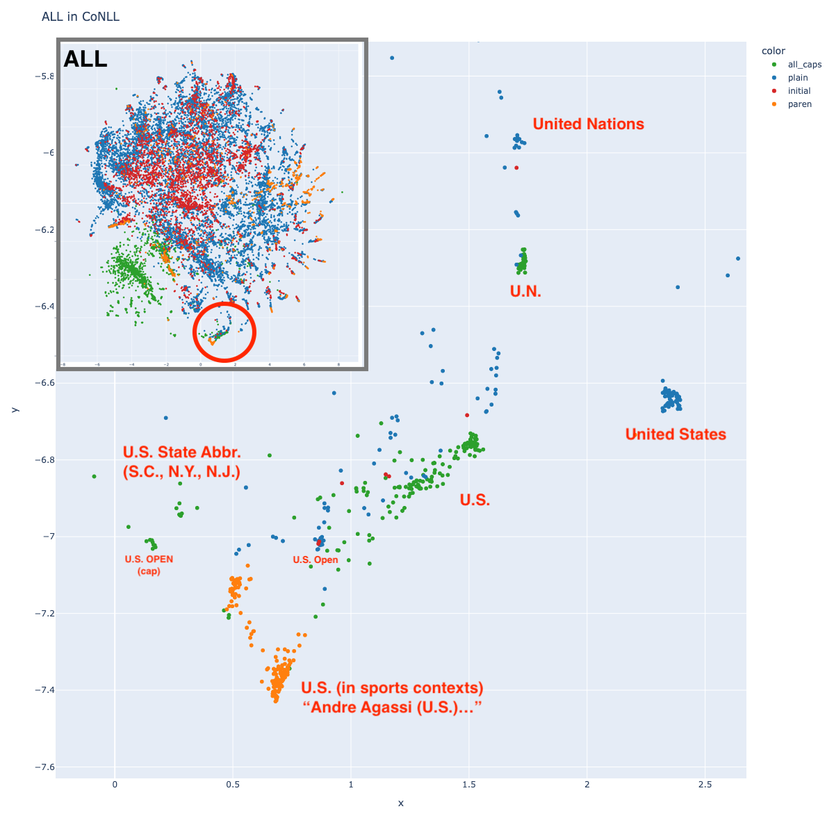
There’s a separate green cluster near point (1, -7) which includes many strings like “U.S.”. Interestingly, this cluster has small satellite clusters containing strings like “U.N.” (United Nations) and “S.C.” (South Carolina), suggesting that the cluster is based on orthography. But there is also a satellite cluster for “United States”, suggesting that entity reference is also sometimes used.

Person

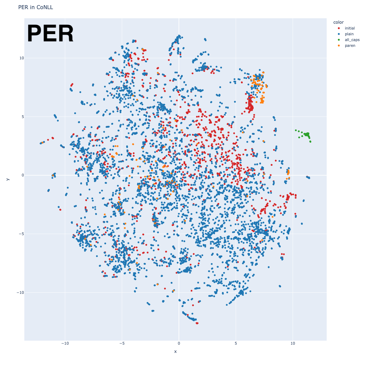
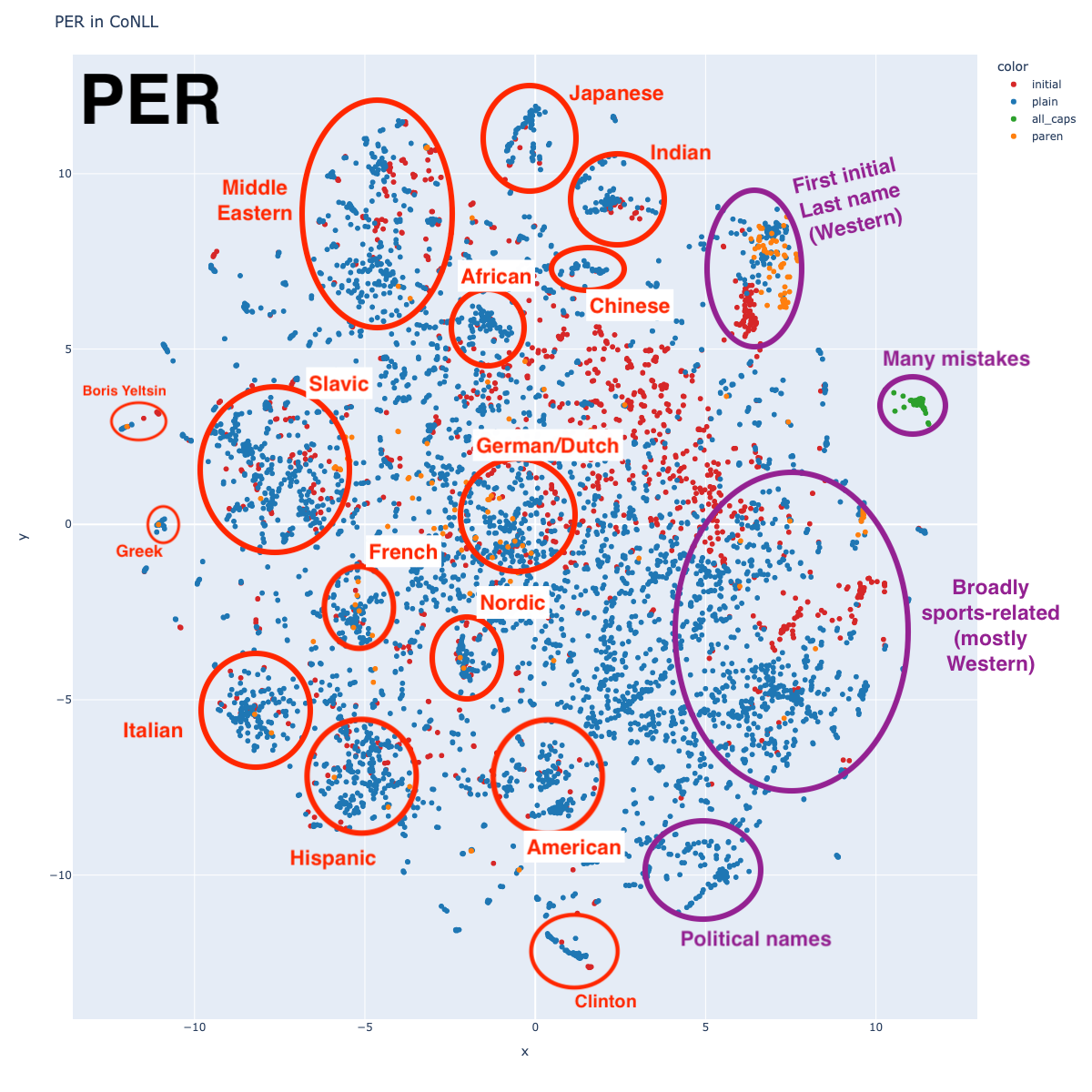
The Person embeddings show some fascinating patterns. They are organized in roughly two sections: on the left half (annotated in red), clusters are formed around nationalities; on the right half (annotated in purple), clusters are more pattern-based. Recall that a non-trivial amount of CoNLL is sports results tables.

The pattern-based clusters include clusters for politics, sports, and then the small group of green dots has many mistakes: including non-persons like “REUTERS”, “DENVER”, and “SAO PAULO”. There are probably other topics in there that I haven’t yet found.

The nationalities clusters are quite distinct. I only marked the major ones (and used very broad categories), but I would encourage you to look around in the interactive map. The clusters get pretty fine-grained.

Why are person names clustered by nationality? There are certainly contextual clues, but my best guess is that the model recognizes component subword patterns, such as those demonstrated below:

Stephen Mayhew → Stephen∙_May∙hew
Yone Kamio → Y∙one∙_Kam∙io
Yelena Gulyayeva → Y∙el∙ena∙_Gu∙ly∙ay∙eva
Etienne Mendy → E∙t∙ienne∙_Mend∙y
Alessandro Baronti → A∙less∙andro∙_Bar∙ont∙i
Juan Carlos Pinero → J∙uan∙_Carlos∙_Pin∙ero
Klimis Alexandrou → K∙lim∙is∙_Alexand∙rou
Sanath Jayasuriya → San∙ath∙_Jay∙as∙uri∙ya

A similar thing happened in MIMICK (Pinter et al 2018), where they explicitly trained subword embeddings for OOV tokens. Their Table 1 shows nearest neighbor examples in English, with “Vercellotti” having nearest neighbors of “Martinelli, Marini, Sabatini, Antonelli” – a pattern very similar to what we see in our plot. The relationship between name string and nationality was also discussed in Poerner et al 2019.

One might also ask: could you recover a world map from these clusters? It’s not a slam-dunk, but if you squint, you can see that American and Hispanic names are close at the bottom, like the North and South American continents. There’s a roughly European section in the middle, and then several Eastern nationalities are grouped together near the top, although it’s all a bit confused (why is India between Japan and China?). This is no Mercator Projection, but it’s not totally random either.

Why might we expect this to work? It seems that BERT groups names according to internal character patterns, which are similar between similar languages. Further, languages that are linguistically close to each other also tend to be geographically close (Heeringa, 2001, Huisman et al 2019). If you follow this (somewhat tortured) line of reasoning, you might expect that distance between clusters correlates with distance between language geographic centers, although there’s no guarantee that the overall placement is consistent with a world map.

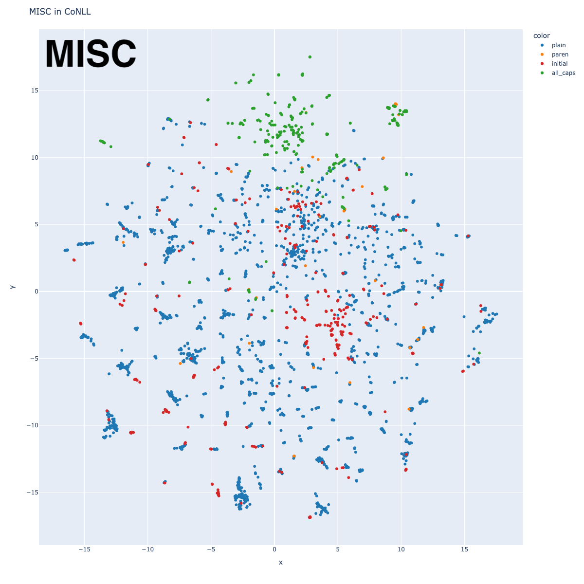
Miscellaneous

The MISC tag in CoNLL is ill-defined, including things as broad as religions, nationalities, slogans, and eras in time. This is reflected in the way that it has no central cluster in the ALL graph. But similar to the Person tags, we see clusters around nationality, as well as political party, and stock exchange.

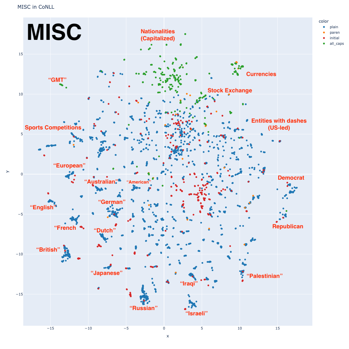
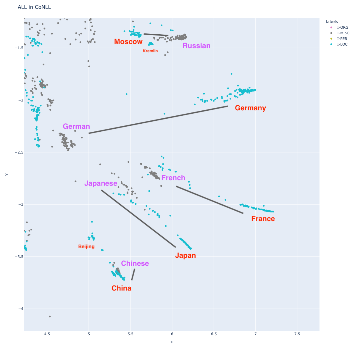Given the way English represents nationalities, one might expect that nationality would be close to the country name (Japanese and Japan, German and Germany, etc.) This turns out to be true. I’ve annotated a few, along with lines representing their cluster distances, but you can find many more such groups. One might ask if it makes sense to tag nationalities with a separate tag from countries.

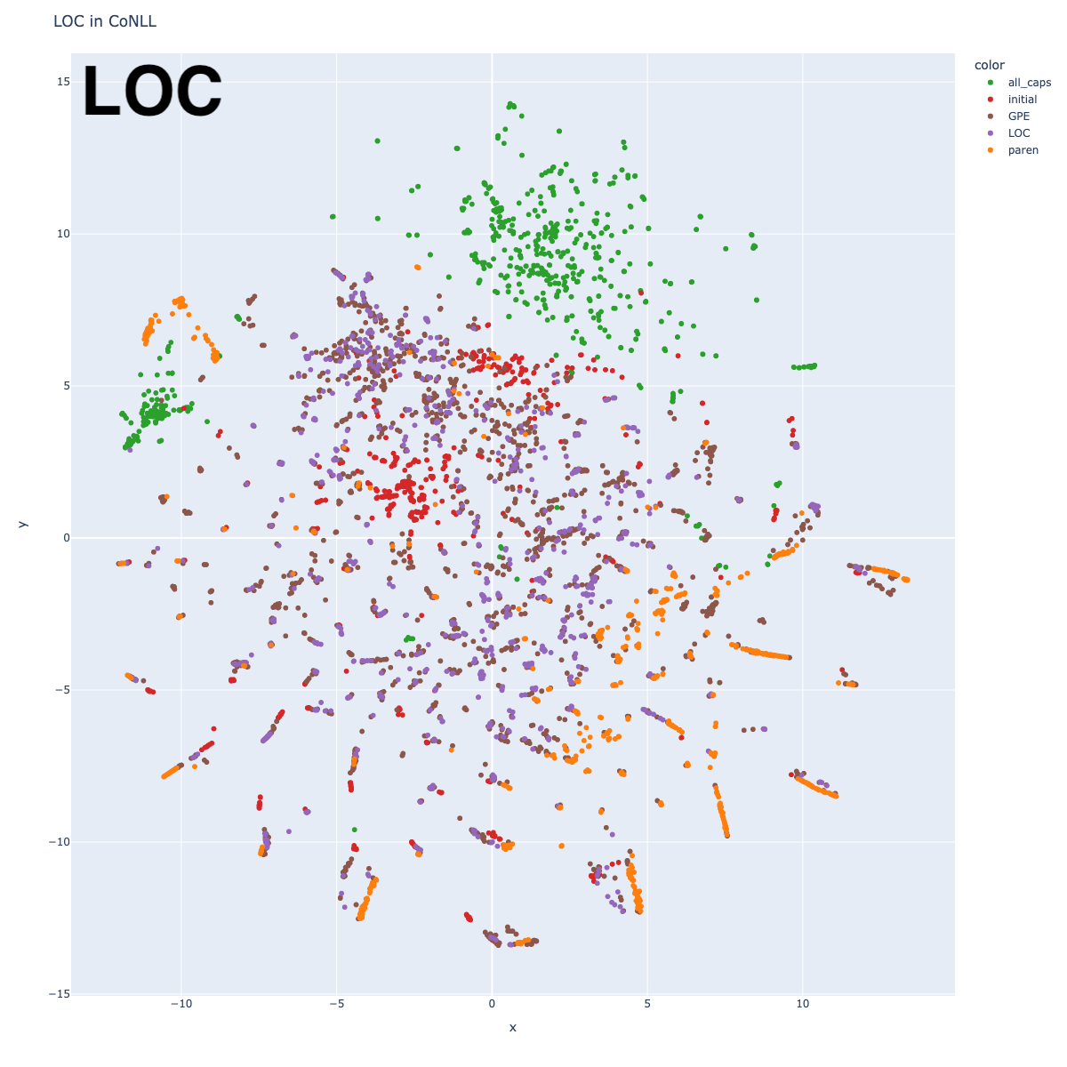
Location

This tag is perhaps the least interesting of all. There are clusters, and they are pretty much all exactly as you would expect: England, Pakistan, Europe, China, Africa, etc. I don’t have a hypothesis about recovering a world map – a glance over it suggests it’s not a close correlation.

There are also clusters at different geographical abstractions: cities, states, countries. Cities that share a country are close to one another, but they are not close to that country. For example, “U.S.” is across the plot from “Chicago.”

My little experiment of trying to distinguish “passive locations” from “locations with agency” (marked as LOC and Geo-Political Entity (GPE), although I think this was a mistake) showed that BERT treats these classes more or less the same. If you find the clusters for “China” (-7, -10), for example, you will find that entities in contexts of “China requested…” or “China said…” (location with agency) are mixed indiscriminately with entities in contexts of “…people in China” or “…traveled to China” (passive location).

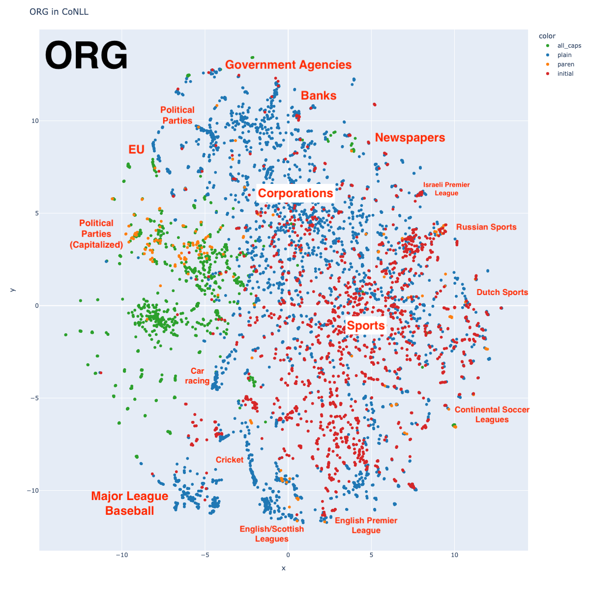
Organization

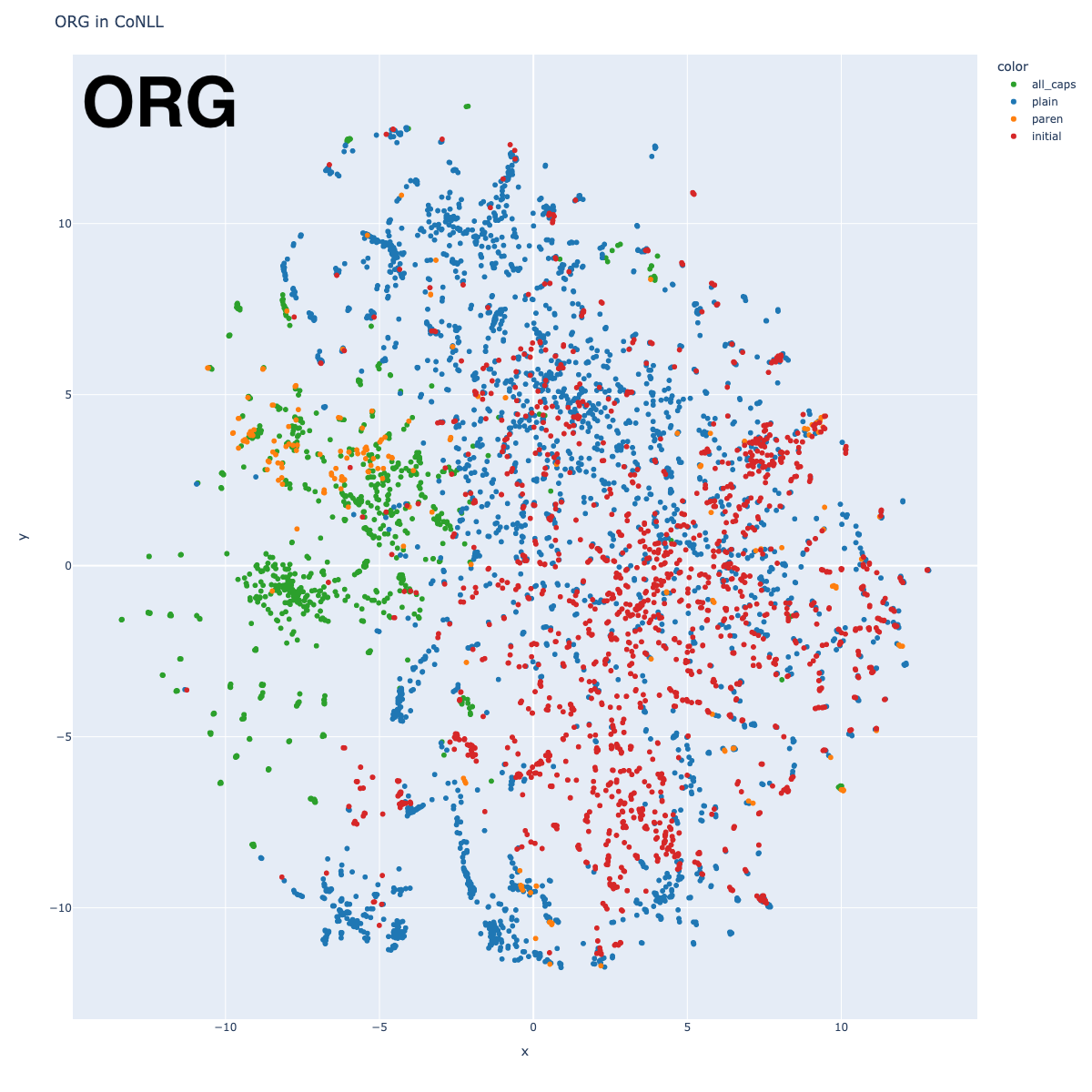
Organizations can be divided in roughly 3 large categories: sports teams (in the bottom half of the graph), governmental agencies and political parties (on the top left edge), and corporations (top right edge). Interestingly, sports teams arrange roughly by league, although not necessarily by sport. Notice how the English Premier League (soccer) is a long way from the Israeli Premier League (soccer).

Conclusions

There’s a whole lot more to be seen in these graphs! I’ve only scratched the surface.

My original goal was to get some intuitions what sorts of relationships entity labels might have with language embeddings. My main conclusions are:

1. There’s no need to separate LOC and GPE
2. The vast majority of the MISC entities are nationalities, which BERT places near the country name. If you tag all nationalities as LOC, you can drop the MISC label.

I’m going to leave it at that. Let me know if you have any comments or insights!

Code can be found in this notebook (tip: open it in Colab and run it on GPU).

Other works

• Naturally, I’m not the first person to study named entity representations in BERT.
• All of this visualization is reminiscent of Datamaps